![]()
Abstract
Each year, college football players hoping to be drafted into the NFL are invited to the NFL Combine. There, players perform certain drills, like the 40 yard dash, vertical jump, and bench press, generating a set of statistics on each player. They also take basic measurements such as height and weight. Our hypothesis was that players with better results would be drafted earlier and have more success in the NFL. Thus, we hoped to be able to predict draft pick number and future success in the NFL based on these metrics. However, we were not able to find any significant relationships between NFL Combine results and either draft position or future career success. Yet there was a significant relationship between future NFL career success and draft position – indicating that NFL teams do indeed draft better players earlier based on factors other than a prospect’s Combine results.
Dataset
We compiled two datasets for our research: one on NFL Combine data from 1999-2015 and another on NFL Draft data from 1999-2015.
The first dataset, of 1999-2015 Combine results, scraped the 2000-2015 results from http://www.pro-football-reference.com/play-index/nfl-combine-results.cgi – this involved copying and pasting the tables from the website which luckily yielded tab-separated values. We used R to clean this data by appending every year’s results into one master file, converting the resulting file into comma-separated values, deleting unnecessary headers (the header row was repeated multiple times throughout the tables), converted height from “feet-inches” string format into inches, deleted an unnecessary column of hyperlinks to “College Stats”, converted the single column of “Team/Round/Pick Number/Year” into four separate columns, and cleaned the “Round” and “Pick Number” columns from string format into integer format (e.g. “4th” into 4).
To add the 1999 NFL Combine data, the oldest we could find, we used Daren Willman’s dataset from his website, http://nflsavant.com/index.php. Luckily, his data was already formatted well. Using R, we simply extracted the relevant columns that matched up with our 2000-2015 dataset and appended it to our master .csv to complete our first full dataset of NFL Combine data from 1999-2015.
Our second dataset is all players who were drafted in the 1999-2015 NFL Drafts with their draft position (team, round, pick number) and their NFL career statistics that can help us measure how successful a player was in the league. We retrieved this data from http://www.pro-football-reference.com/draft/, year-by-year from 1999-2015. We downloaded the comma separated value file for a given year’s draft results and appended all 17 years’ worth into one master file. We then cleaned the data by deleting unnecessary headers (the header row was repeated multiple times throughout the tables), renamed some headers for clarification purposes (e.g. differentiating Passing Touchdowns from Rushing Touchdowns), and deleted an unnecessary column of hyperlinks to “College Stats”.
However, not all players who were drafted in those years participated in the Combine, and not all players who participated in the Combine were drafted into the NFL. Thus, we had to match the players’ combine statistics to their Draft and career data.
In order to do this, we imported the data into Microsoft Excel, and wrote a macro to integrate the two datasets. Essentially, the macro performed a left outer join on the NFL Combine dataset with the NFL Draft dataset, matching on draft year and overall draft pick number. Specifically, we used two nested for loops; the first went through all the players in the combine and selected their draft year and overall draft pick number, while the inner loop went through all the draft data looking for an entry with matching draft year and overall draft pick number. When a match was found, the macro added the data from the draft table to the combine entry for the player and broke out of the inner for loop, moving onto the next combine entry.
The result was a dataset with 3,795 players who participated in the Combine and were subsequently drafted, along with 1,806 players with only Combine data who were never drafted. In all, our final integrated dataset included 5601 players with 39 variables. Notable variables include all 6 NFL Combine drills (40 Yard Dash, Bench Press, Vertical Jump, Broad Jump, Three Cone Drill, Shuttle Run), position-specific career metrics (e.g. Rushing Yards, Receiving Touchdowns, Tackles), miscellaneous variables (e.g. Position, Team Drafted By), and our “success” metric, Career Approximate Value (Career AV).
Approximate Value is a widely-used advanced football metric, independent of position, that measures the value a player contributes to their team during a season. Career Approximate Value (Career AV) is a weighted sum of a player’s season-by-season Approximate Values, where their best season is unweighted, the second best season is weighted at 0.95, their third best weighted at 0.9, and so on. This weighting scale values players who have had at least one exceptional season over those who have consistently average seasons. We specifically defined “success” in the NFL to be Career AV divided by seasons in the league in order to avoid penalizing currently active players to allow us to be able to make cross-generational comparisons.
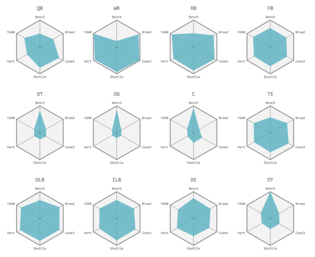
We explored the NFL Combine data by finding the “shape” of NFL prospects, grouped by position. In the visualization we sought to determine how different positions varied in their performance on Combine drills. The six points of each hexagon represent six different Combine measurements. The six points of the blue hexagon represent the average performance of players from a given position on each drill. Better performance, also interpreted as greater athleticism, is indicated by a more expansive hexagon.
There are several interesting patterns we noticed from this exploration. Wide receivers and cornerbacks have very similar shapes, confirming the notion that they have similar athletic builds given that cornerbacks’ primary role is to guard wide receivers. Free safeties also have similar shapes to cornerbacks and wide receivers, given that they often serve as backup to cornerbacks for guarding wide receivers. Strong safeties and free safeties are similar as they play near-identical roles, except for the fact that strong safeties often assist in run defense – explaining their slightly higher bench performance as an indicator of the strength necessary to stop the run. Some positions are extremely specialized, namely offensive linemen and defensive tackles who primarily need to have extraordinary strength, seen in their bench press, and little else as far as other Combine measurements which leads to their “pointy” hexagonal shape. Lastly, other positions are less specialized, i.e. shaped closer to a regular hexagon. Fullbacks, tight ends, and outside/inside linebackers all have fairly balanced measurements. This agrees with their versatile usage on the field, where they must assume the roles of several more specialized positions (e.g. fullbacks must be able to proficiently block, run, and catch the ball).
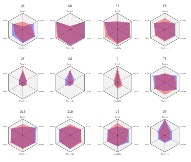
Additionally, we compared the “shape” of the top players at each position (specifically, the top 10 based on Career AV per Season) against the average for their respective position. The red areas represent the average player’s Combine measurements and the blue areas represent the top players.
There are noteworthy differences for several positions. Top quarterbacks appear to be exceptionally more athletic than average, which can be influenced by mobile “dual-threat” quarterbacks who are skilled runners in addition to passers. Top offensive guards appear to be more athletic and less one-dimensional than average guards, which can be explained by the athletic expectations of an offensive guard to be able to “pull” from one side of the line to another on run plays – requiring lateral quickness and overall greater athleticism. The same could be said for outside linebackers, defensive ends, and defensive tackles where exceptional athleticism is present in the top players, differentiating them from the crowd. Lastly, top tight ends are also more athletic than average, which aligns with the fact that pass-catching tight ends require greater physical versatility and provide far greater value to their team beyond blocking.
Methodology and Results
We explored the pairwise relationships between three different quantities: Combine results, success in the NFL as measured by Career AV per season, and draft pick position. First, by determining if there is a strong or weak correlation between Combine results and career success, we could determine how teams should factor in the combine results when drafting players. Second, if combine results are related to draft pick, teams would be able to predict how early players they are interested in would be drafted, allowing them to strategize accordingly. Lastly, by exploring the relationship between career success and draft pick position, we would be able to compare the value of different draft picks; for example, how much better it is for a team to have the first overall draft pick versus the fifth overall pick.
Combine Results and NFL Success
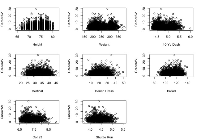
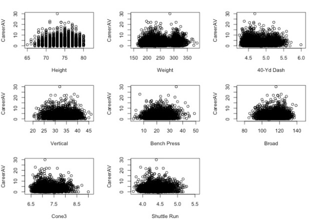
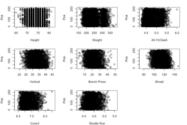
Due to the importance of athleticism in football, we hypothesized that NFL success could be predicted by combine results. First, to determine the feasibility of building a predictive model, we began by investigating correlations between each individual statistic from the Combine and Career AV per season. Unfortunately, the scatterplots below revealed that there were no clear relationships. Correlation coefficients ranged from -0.15 to 0.12, suggesting that there were no linear associations.
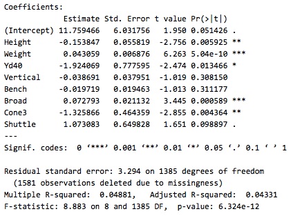
Despite our scatterplot and correlation results suggesting that the relationship between individual statistics and career success was weak, we trained a linear regression model using all Combine results to predict Career AV per season. We thought that perhaps this model would capture dependencies between different Combine drills that interact to predict success, even though individual drills were not highly correlated. The results are shown in the following graphic.

To our disappointment, the low R-squared value indicates that our regression model was a very poor fit. It was only able to predict 4% of the variation in Career AV per season. Additionally, although some of our coefficient estimates were statistically significant, we doubt their accuracy, since some suggested that worse Combine performance (i.e. slower 40-yard dash and 3-cone drill times) would lead to better Career AV per season.Therefore, we concluded that Career AV per season could not be predicted purely by Combine results.
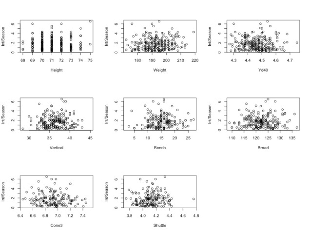
However, based on our exploratory visualization of different positions combine results, we knew that different combine drills are more important for different positions. Thus, we suspected that splitting up players by position before predicting success would yield better results. Unfortunately, splitting by position yielded no significant relationship between Combine results and Career AV per season. We also tried using different predictors for success for different positions, such as tackles per season for linebackers and passing yards per season for quarterbacks. We again investigated the correlation between individual combine drill results and position specific success metrics, but found no significant relationship. For example, the scatter plot below shows the lack of correlation between cornerbacks’ combine results and interceptions per season.
Based on these poor results, we concluded that NFL success could not be predicted by Combine results. Thus, teams should not factor in the Combine when determining which players to draft, but should instead focus on other measures of ability such as college performance or traditional qualitative player scouting.
Combine Results and Draft Pick Position
We also hypothesized that players that did better in the Combine would be drafted earlier, since the Combine is supposed to be a tool for teams to evaluate potential picks. However, the following scatter plot of individual combine results versus draft pick number shows no correlation.
This visualization shows that draft pick positions are spread relatively uniformly across all levels of combine performance. Splitting up by position also yielded similarly uncorrelated results. This is unsurprising given our previous conclusion that Combine results do not predict future success in the NFL. If coaching staffs and front offices know that the Combine does not predict success, then there is no reason for them to use it to choose when to draft players either.
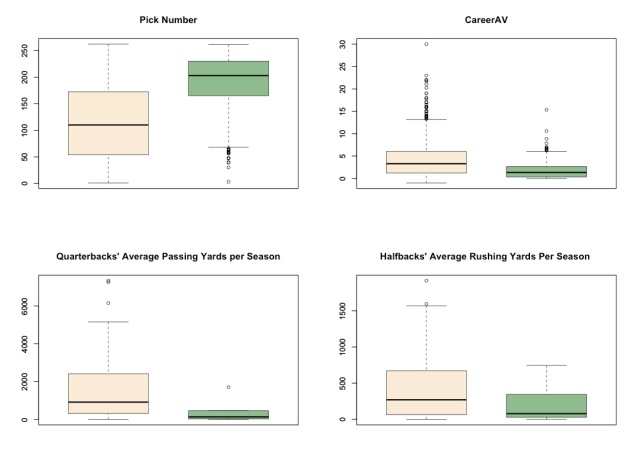
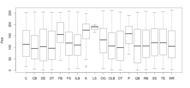
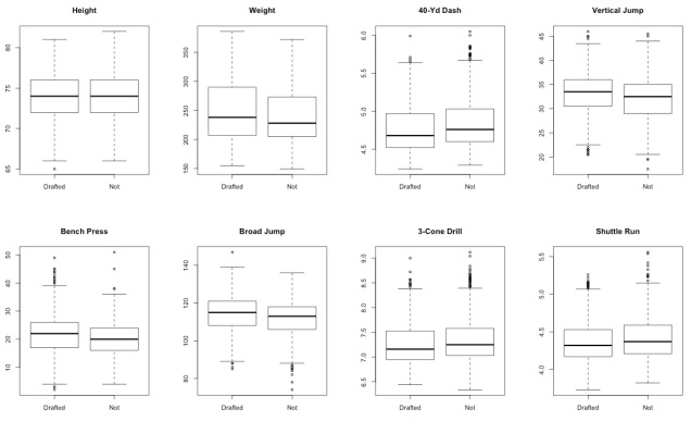
We further explored this result by examining the subset of players who attended the Combine but did not get drafted, comparing their results on the Combine drills to participants who did get drafted. There were no significant differences between groups, as can be seen in the following box and whisker plot. The distribution of results in each drill appears to be the same between drafted and non-drafted combine participants. This further supported our conclusion that coaches do not take into account the Combine when determining who to draft.
Draft Pick Position and NFL Success
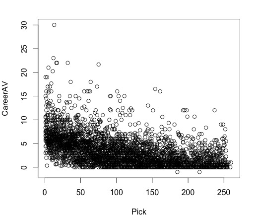
Based on background knowledge of the NFL, we hypothesized that better players do get drafted earlier. Looking at a basic scatter plot of pick number versus Career AV per season, this hypothesis was supported.
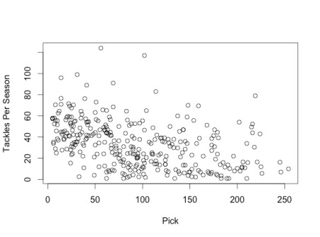
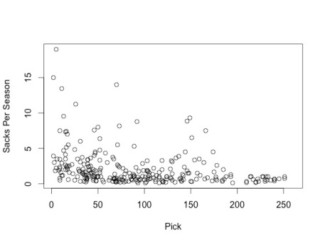
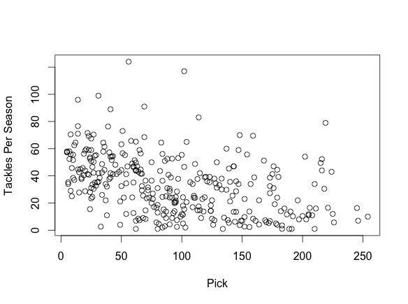
We also determined that players drafted earlier would have better career performance measured not only by Career AV per season, but also by position-specific metrics. We created scatterplots for multiple position-specific metrics vs. pick number and found that earlier picks did tend to have stronger NFL performances. We include two scatterplots as example evidence:
This first graph plots cornerbacks’ average tackles per season vs. pick number.
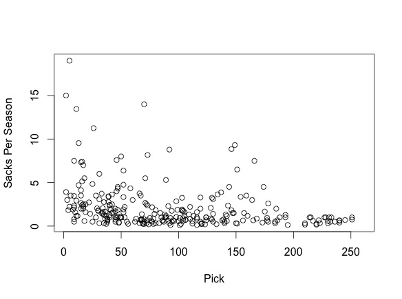
This second graph plots linebackers’ average sacks per season vs. pick number.
We decided to formalize the correlation between Career AV per season and draft pick number further by assigning each pick number a “value” based on how well players drafted in that position have historically done compared to those drafted before and after them.
The most famous draft pick valuation was done by Cowboys’ coach Jimmy Johnson in the 1990s to help his team’s management decide how to properly evaluate trades involving draft picks. For example, he valued the #1 overall pick at 3000. This means that under his system, trading away the #1 pick requires a return draft picks whose total value is greater than or equal to 3000 (for example, the third overall pick valued at 2200 grouped with the twentieth overall pick valued at 850 – a trade with a net of +50 value).
It must be noted that Coach Johnson did not use any rigorous statistics to support his pick valuation. Indeed, his valuation has been heavily critiqued since then, and thus we decided to compare our results to his and see if we agree with the critics.
First, we grouped together players by draft pick number, and averaged the Career AV per season across all players in each group. We did not include players drafted in 2015 or 2016, since there is not yet enough data to infer how well they will truly perform in the NFL. Thus, for most pick numbers, we had 16 players drafted in that position in the years between 1999 and 2014.
When analyzing any type of sports data, sample bias is very important to consider. Better players are given more playing time and thus accumulate better metrics to measure the value they add to their team. This leads to a non-representative sample from the population of NFL players as worse players who are given less to no playing time are under-represented. In order to take into account players who did not last an entire season in the NFL – an important group of draft “busts” that must be represented – we give them a Career AV per season of 0 to indicate the absence of value added to their team.
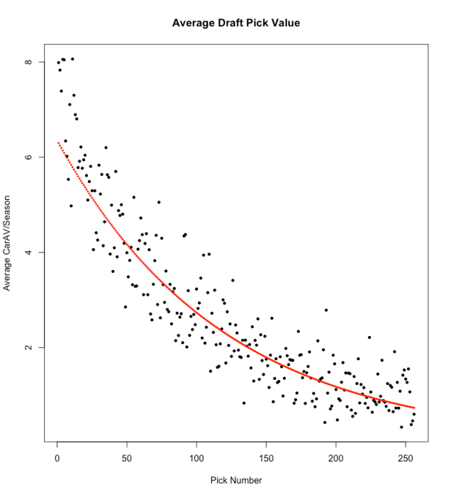
Above, we plotted the Average Career AV per Season for each individual pick number across the 16 drafts in our dataset. A non-linear inverse relationship is evident in the scatter plot. Using a log transformation of the dependent variable, we ran a linear regression to find the best-fit line through these points. This yielded a statistically significant model where a substantial 81.2% of the variation in the log(Average Career AV per Season) was predictable by Pick Number.
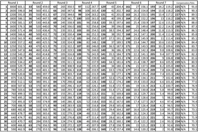
We then used this model to generate a new valuation of each pick position in a draft and compared this to Jimmy Johnson’s original values in the following graph for easy visual comparison. To facilitate comparison, we scaled our values so that the sum of picks 1 to 224 was equal between the two systems. For exact numbers in our and Jimmy Johnson’s valuations, see Appendix A.
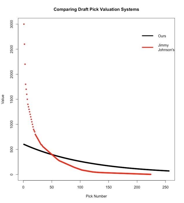
Compared to our valuation, Jimmy Johnson severely overvalued early picks and also undervalued later picks. However, while our valuation is based in quantitative analysis unlike Coach Johnson’s, we neglect to take into account factors like a specific team’s desire for players of a specific position. For example, if two teams are both weak at the quarterback position and there is one standout quarterback in the draft, having the higher draft pick of the two is far more important than pure Career AV per season would indicate. Thus, it is likely that the true valuation is somewhere between the two systems.
Conclusion
We concluded that, contrary to our hypothesis, Combine results alone cannot accurately predict either draft pick or eventual success in the NFL. This result was frustrating, because we had hoped to create a predictive model to grade future NFL drafts. However, better players do get drafted earlier, implying that coaches look at other indicators, such as college statistics or traditional qualitative scouting, to identify better players. While pure physical ability is important in football, it seems that all players who are capable of playing at the highest levels have sufficient athleticism, and what really matters are intangibles like situational awareness and on-field decision making – actual football skills. Thus, according to our analysis, the Combine alone is not a useful event for evaluating talent.
There are several opportunities for further exploration and analysis to be done on evaluating the NFL Draft. Although we failed to find a relationship between the Combine and career success, it is worth exploring the integration of college performance and other qualitative analyses such as sentiment analysis of traditional scouting reports into a predictive model. Both this and a similar model to predict when a player will be drafted would be of great use to an NFL franchise when preparing and participating in the entire NFL Draft process.
Additionally, draft pick valuation could be extended to better reflect reality. There are inequalities in how different positions are valued in the league, such as quarterbacks being valued more than usual due to their important leadership role in an offense, and these deviations could be integrated into the valuation system. This valuation system could also be extended to reflect the different year-to-year positional needs of each team – a dynamic model that could be tailored to a specific year that could help a team more accurately value draft picks when considering trades.
Appendix A
In the following chart, for each round of draft picks, the first column is the pick number, the second is Jimmy Johnson’s valuation of that pick, and the third is our valuation.